Trajectory Forcing: Exploiting Diffusion Trajectories for Autoregressive Long Video Generation

Selected qualitative examples. Compare this scene

Bohan Wang^*
Shuo Chen^*
Yunzhi Li^*
Zhaozheng Chen
Junzhe Zhang
Hanwang Zhang^†

Huawei Noah Research Institute

* Equal contribution. † Corresponding author.

01Idea

Denoising trajectories are context for what comes next.

Trajectory Forcing turns intermediate denoising predictions into useful context for generating subsequent video chunks, across supervised training and self-rollout training.

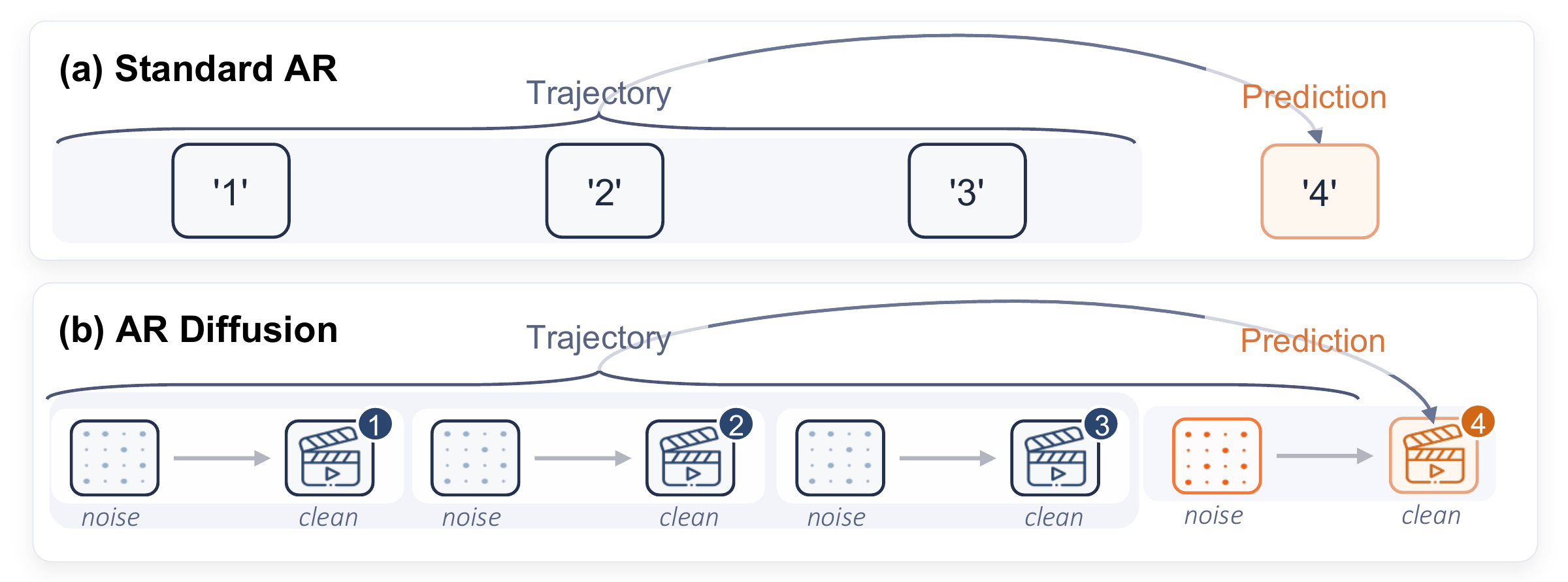
Paper figure. (a) Standard autoregression: tokens 1, 2 and 3 form the history used to predict token 4. (b) Autoregressive diffusion: each chunk is generated from noise to clean through several steps, so chunks 1 to 3 each carry a trajectory that conditions the prediction of chunk 4. — (a) Tokens are generated as single units. (b) Video chunks leave a history of denoising predictions.

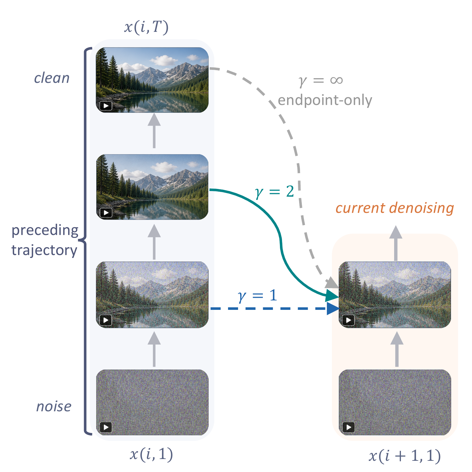
Conceptual view Endpoint-only conditioning uses each earlier chunk’s final output; trajectory conditioning also draws on intermediate predictions.

Each column is one chunk’s denoising trajectory, from Gaussian noise at the top to its final output at the bottom.

In this conceptual view, the shaded history includes complete earlier trajectories and the current chunk’s earlier states. The arrow shows how this history conditions the current update. The current chunk’s initial noise is sampled without conditioning.

In practice, each update uses one selected clean-signal prediction from each retained preceding chunk. Selection details.

02METHOD

From trajectory learning to practical conditioning

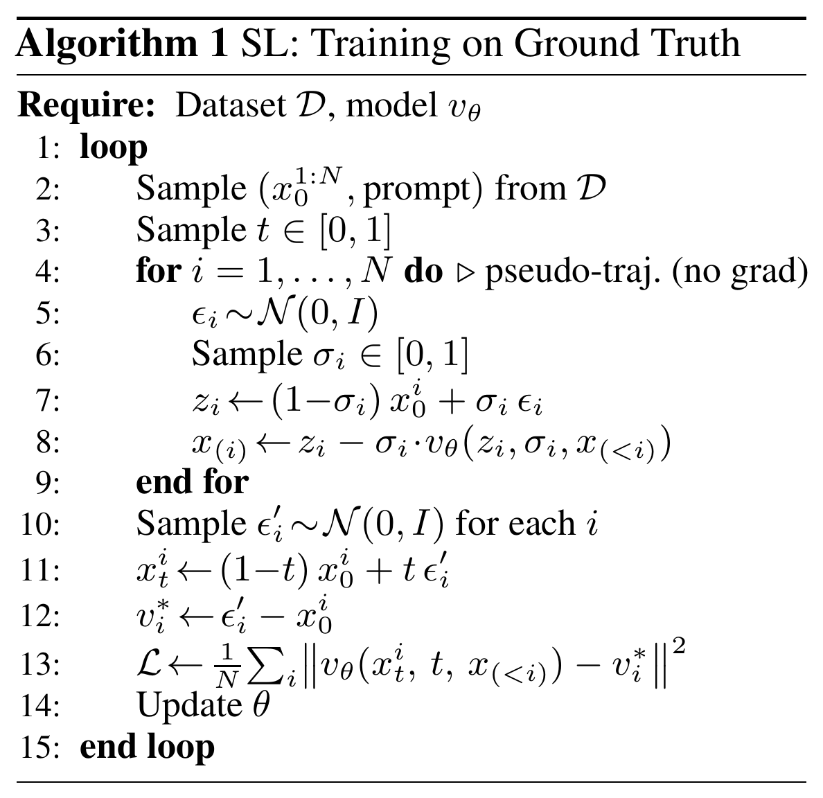
Ground-truth videos have no model-generated denoising history, so TraF learns in two stages: pseudo-trajectories first, then trajectories from its own rollouts.

Stage 1 · SL

Pseudo-trajectories from ground truth

Source: Ground-truth videos
Context: At a sampled noise level, one velocity prediction per chunk gives a clean-signal estimate. Sampling different noise levels across training yields the pseudo-trajectory points.
Objective: Flow matching

Algorithm 1 pseudo-code from the paper

Algorithm 1 from the paper, SL: training on ground truth. For each chunk, sample a noise level, interpolate with Gaussian noise and use one velocity prediction to estimate the clean signal without gradients. Then train the model with flow matching to predict velocities for freshly noised chunks using those estimates as context.

Stage 2 · RL

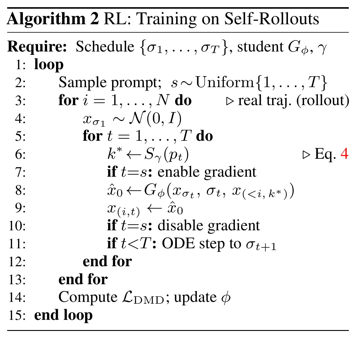
Real trajectories from self-rollout

Source: Initialized from the SL model, the student generates chunks autoregressively with a four-step self-rollout
Context: Its four denoising predictions form each chunk’s real trajectory; selected predictions condition later chunks
Objective: Distribution Matching Distillation (DMD) with a frozen teacher and a learned critic

Algorithm 2 pseudo-code from the paper

Algorithm 2 from the paper, RL: training on self-rollouts. For each chunk, run the denoising schedule; at each step select trajectory context from preceding chunks, predict the clean signal, and cache it in the trajectory; then compute the DMD loss and update the student.

Selection · practical conditioning

Using trajectory context efficiently

Full-trajectory conditioning adds attention and memory cost. TraF uses one selected prediction per retained preceding chunk at each update.

Paper figure. Left: clean-signal estimates predicted at successive denoising steps of a preceding chunk. Right: the current chunk being denoised, which receives one of the preceding chunk's intermediate estimates as context. Arrows illustrate the selection options shown in the paper. — A preceding chunk’s trajectory supplies context to the current update. Arrows are illustrative, not a timestep mapping.

Cache: Clean-signal predictions from preceding chunks, not noisy latents.
Context: One selected prediction from each retained preceding chunk at each denoising update.
Rule: On the finite denoising grid, select the available prediction nearest to the regularized target progress.

Selection rule continuous target & discrete steps

The continuous target scales the current step’s amplitude signal-to-noise ratio by γ.

S_γ(p) = γp1 + (γ − 1)p

p = 1 − σ is denoising progress, from noise (0) to clean signal (1); γ ≥ 1.

On the finite grid, TraF adds a regularization term to the target ratio and converts it to progress before selecting the nearest available prediction. See Appendix A of the paper.

γ = 1 is step-aligned. γ → ∞ approaches endpoint-only conditioning.

03Results

Trajectory context for long video generation

We first examine 30-second generation, then generation at TraF’s five-second training duration. These comparisons from the paper span different model and training configurations.

Indigo row markers identify Self Forcing, Causal Forcing and TraF. See their training and inference settings.

Two evaluation settings. Different prompt sets and scoring protocols: the 5-second and 30-second scores are not directly comparable.

30-second generation

6× TraF’s training duration

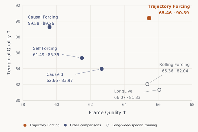
We evaluated each method on the same 128 MovieGenBench prompts. Nine VBench dimensions are grouped into Temporal Quality, Frame Quality and Text Alignment; Total is the equal-weighted average of these three axes.

Scatter plot of Frame Quality and Temporal Quality for six methods in the 30-second evaluation: CausVid, Causal Forcing, Self Forcing, Trajectory Forcing, Rolling Forcing and LongLive. Hollow markers identify Rolling Forcing and LongLive, which use long-video-specific training. — 30-second evaluation. Frame Quality and Temporal Quality are higher-is-better. Labels show Frame / Temporal scores. Axes are zoomed; hollow markers denote long-video-specific training.

30-second VBench axes, total score, VideoScore2 and Quality Drift for six selected methods, with long-video-specific training shown as a separate group.
Method	Total ↑	Temporal Quality ↑	Frame Quality ↑	Text Alignment ↑	VideoScore2 ↑	Quality Drift ↓
Main comparisons
CausVid1.3B · Wan-14B teacher	68.50	83.97	62.66	58.88	3.549	2.72
Causal Forcing1.3B · Wan-14B teacher	70.48	89.26	59.58	62.61	3.589	4.36
Self Forcing1.3B · Wan-14B teacher	71.06	85.35	61.49	66.33	3.719	2.21
Trajectory Forcing Ours1.3B · Wan-14B teacher	73.98	90.39	65.46	66.08	3.771	1.38
Long-video-specific training
Rolling Forcing1.3B · Wan-14B teacher	71.39	82.04	65.36	66.77	3.804	0.56
LongLive1.3B · Wan-14B teacher	71.48	81.33	66.07	67.04	3.801	0.60

Rolling Forcing and LongLive use long-video-specific training and their own inference architectures. SF, CF and TraF use the same sliding-window inference with an attention sink in this evaluation.

TraF’s 30-second Total is 2.92 points higher than Self Forcing (95% paired prompt-bootstrap CI: +2.06 to +3.78).

Quality Drift is the absolute imaging-quality difference between the first and last 5-second segments; lower is better. VideoScore2 reports its text-alignment sub-score. All other columns are higher-is-better.

Bold marks the best value in each column across all displayed methods. TraF leads Total and Temporal Quality; LongLive leads Frame Quality and Text Alignment; Rolling Forcing leads VideoScore2 and has the lowest Quality Drift. See the paper for all methods.

5-second generation

VBench · short video

946 prompts, all 16 VBench dimensions. Total = (4 × Quality + Semantic) / 5. Throughput and latency are reported in FPS and seconds, respectively.

5-second VBench scores and inference speed for twelve selected methods across three model categories.
Method	Total ↑	Quality ↑	Semantic ↑	Throughput ↑FPS	Latency ↓seconds
Bidirectional Video Diffusion
LTX-Video1.9B · Teacher —	79.83	81.88	71.62	8.98	13.5
Wan2.1-1.3B1.3B · Teacher —	83.37	84.30	79.65	0.78	103
Autoregressive Video Diffusion
MAGI-14.5B · Teacher —	78.88	81.67	67.72	0.19	282
NOVA0.6B · Teacher —	80.31	80.66	78.92	0.88	4.1
Pyramid Flow2B · Teacher —	80.75	83.41	70.11	6.70	2.5
SkyReels-V21.3B · Teacher —	81.97	83.96	74.01	0.49	112
Distilled Autoregressive Video Diffusion
CausVid1.3B · Wan-14B teacher	81.33	83.98	70.72	17.0	0.69
Rolling Forcing1.3B · Wan-14B teacher	83.07	83.61	80.89	15.8	0.76
LongLive1.3B · Wan-14B teacher	83.09	83.69	80.69	18.0	0.65
Causal Forcing1.3B · Wan-14B teacher	84.04	84.59	81.84	17.0	0.69
Self Forcing1.3B · Wan-14B teacher	84.31	85.07	81.28	17.0	0.69
Trajectory Forcing Ours1.3B · Wan-14B teacher	85.15	85.89	82.20	15.0	0.78

We evaluated TraF, Rolling Forcing and LongLive. The Self Forcing row comes from its original paper. The other rows shown here come from the Causal Forcing paper. See the full table and sources in the paper.

Bold marks the best reported value in each column. Among the methods shown, TraF leads on Total, Quality and Semantic. LongLive has the highest reported throughput and lowest reported latency.

SF / CF / TraF setup

Base model: Wan2.1-T2V-1.3B
Inference: 4 steps
Resolution: 832×480
Video frame rate: 16 fps

Self Forcing, Causal Forcing and Trajectory Forcing use the same backbone architecture and teacher during RL. TraF starts from its SL checkpoint, while SF and CF use their original initializations. In the 30-second evaluation, all three use the same sliding-window inference with an attention sink.

The following three ablations examine the information in trajectory context, learning before distillation, and the choice of conditioning predictions.

Evidence · 5-second VBench

Testing the information in trajectory context

Adding Gaussian noise to endpoint predictions lowers Total at both tested magnitudes. The unperturbed endpoint scores 84.24.

VBench Total ↑ higher is better

Gaussian σ = 0.22: 83.87
Gaussian σ = 0.11: 83.95
Trajectory predictions: 85.15

View all three VBench metrics

5-second VBench ablation. Endpoint predictions with added isotropic Gaussian noise serve as the context for the two noise controls. All three metrics are higher-is-better.

5-second VBench noise versus trajectory ablation.
Context	Total ↑	Quality ↑	Semantic ↑
Noisy endpoint, σ = 0.22	83.87	84.76	80.29
Noisy endpoint, σ = 0.11	83.95	84.92	80.08
Trajectory	85.15	85.89	82.20

Training evidence

SL stage, before distillation

Same architecture and data, evaluated before distillation with 50-step denoising on 5-second VBench. All three metrics are higher-is-better.

SL-stage ablation before distillation, evaluated with 50-step denoising.
SL strategy	Total ↑	Quality ↑	Semantic ↑
Teacher Forcing	83.47	84.09	81.02
Diffusion Forcing	84.07	84.66	81.68
Trajectory	84.39	85.25	80.96

Trajectory has the highest Total and Quality; Diffusion Forcing has the highest Semantic score. These SL-stage scores use a different evaluation stage and denoising schedule from the final four-step model.

Conditioning evidence

Choosing trajectory context

5-second VBench full-pipeline ablation. Each γ setting uses a separately trained and evaluated model. See Figure 2 of the paper. All three metrics are higher-is-better.

5-second VBench full-pipeline selection ablation from Figure 2.
γ	Total ↑	Quality ↑	Semantic ↑
1	84.82	85.49	82.10
2	85.15	85.89	82.20
3	85.13	85.91	81.97
5	84.58	85.47	81.03
10	84.62	85.40	81.50
∞	84.24	85.04	81.07

Every finite γ reported here has a higher Total than endpoint-only conditioning (γ → ∞). γ = 2 and 3 give the highest Total scores. Bold marks the best value in each column.

04Videos

30-second comparisons

Selected qualitative examples from SF, CF and TraF, played together at the original speed.

0:00 / 0:30

Prompt

The comparison plays the first 30 seconds of each video at original speed. “Full video” opens the complete file. Comparisons with other methods are in the paper.

Enable JavaScript for synchronized comparisons. All nine videos remain available directly. Pigeon: Self Forcing, Causal Forcing, TraF. Portrait: Self Forcing, Causal Forcing, TraF. Animated film: Self Forcing, Causal Forcing, TraF.

05Cite

BibTeX

Download .bib

@inproceedings{wang2026trajectoryforcing,
  title     = {Trajectory Forcing: Exploiting Diffusion Trajectories for
               Autoregressive Long Video Generation},
  author    = {Wang, Bohan and Chen, Shuo and Li, Yunzhi and
               Chen, Zhaozheng and Zhang, Junzhe and Zhang, Hanwang},
  booktitle = {Advances in Neural Information Processing Systems},
  year      = {2026}
}